Logistic model of population dynamics is one of the best examples of how simple ODE can be used to describe many phenomena with decent accuracy. It was first proposed by Verhulst and can be written as follows

$y' = r y\left(1-\frac{y}{K}\right)$,

where $y=y(t)$ is the population of certain species at time $t$, $r$ is characteristic growth coefficient and $K$ is the so-called environmental capacity. For $K\rightarrow\infty$ we obtain the exponential Malthus model. Logistic equation states that we are dealing with a population which growth rate, i.e. $y'$, is proportional to the number of organisms. However, the growth of the population is slowed by the environmental capacity - when $y$ is close to $K$, the derivative $y'$ almost vanishes. In reality, this can be achieved by various reasons such as lack of food or spatial limitations. Logistic model is probably the simplest with these features.

Let us see how does this model perform in reality. As an example, we will analyse the data describing the population of New York form 1746 to 2014 (a very long timespan!).

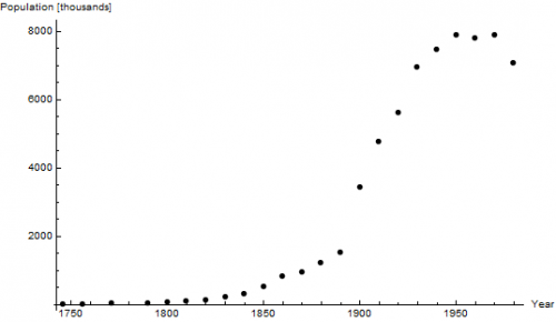
We see that initially, population grows exponentially and then, around 1950, becomes saturated. As one can be easily convinced, there is a multitude of reasons for such a behaviour and we cannot deal with each of every one of them at a time. Instead, we expect that, overall, many of those factors lead to an average behaviour described by some simple model. Surprisingly, this is often the case.

A quick calculation shows that the solution of logistic equation can be written as

$y(t) = \left(\frac{1}{K}+\left(\frac{1}{y_0}-\frac{1}{K}\right)e^{-rt}\right)^{-1}$,

where $y_0$ is the initial population. We use Mathematica to calibrate our model on the NY data. That is, to find $K$ and the growth coefficient $r$ we enter

$FindFit[dataNY, 1/(1/K + (1/y0 - 1/K) E^{(-r (t - t0)))}, \left\{\left\{r, 0.04\right\}, \left\{K, 8000\right\}\right\}, t]$

and we get

${r \rightarrow 0.0463894, K \rightarrow 8248.62}$.

Notice that it is wise to give your computer some hint where to look for a solution. Least-squares method is a brilliant one but, in our case, it reduces to solve a nonlinear minimization problem which can have many solutions (if any). More information we enter, the better the result. Do not treat your computer as an all-knowing black box that always spits out correct results. This is simply not true. Computers are programmed by people (as for year 2020) and every user should be aware of the software which he uses for his calculations. Do not be ignorant.

Our modelling of NY data yields a very nice plot (in log-log coordinates for clarity).

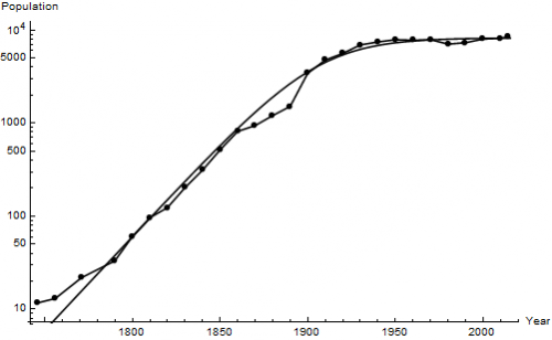
Of course, this is not a perfect fit, but in real-world applications we cannot expect miracles from a simple model taught to undergraduates!